Spherical coordinates and harmonics

3.2 Spherical coordinates and harmonics

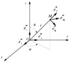
Spherical coordinates (see Figure 19

) are well adapted for the study of many problems in numerical relativity. Those include the numerical modeling of isolated astrophysical single objects, like a neutron star or a black hole. Indeed, stars’ surfaces have sphere-like shapes and black hole horizons have this topology as well, which is best described in spherical coordinates (eventually through a mapping, see Section 3.1.1). As these are isolated systems in general relativity, the exact boundary conditions are imposed at infinity, requiring a compactification of space, which is here achieved with the compactification of the radial coordinate $r$ only.

Figure 19: Definition of spherical coordinates $(r,𝜃,φ)$ of a point $M$ and associated triad $(⃗e ,⃗e ,⃗e ) r 𝜃 φ$ , with respect to the Cartesian ones.

When the numerical grid does not extend to infinity, e.g., when solving for a hyperbolic PDE, the boundary defined by $r = const$ is a smooth surface, on which boundary conditions are much easier to impose. Finally, spherical harmonics, which are strongly linked with these coordinates, can simplify a lot the solution of Poisson-like or wave-like equations. On the other hand, there are some technical problems linked with this set of coordinates, as detailed hereafter, but spectral methods can handle them in a very efficient way.

3.2.1 Coordinate singularities

The transformation from spherical $(r,𝜃,φ)$ to Cartesian coordinates $(x,y,z)$ is obtained by

x = rsin𝜃 cosφ, (90 ) y = rsin𝜃 sin φ, (91 ) z = rcos 𝜃. (92 )

One immediately sees that the origin $r = 0 ⇐ ⇒ x = y = z = 0$ is singular in spherical coordinates because neither $𝜃$ nor $φ$ can be uniquely defined. The same happens for the $z$ -axis, where $𝜃 = 0$ or $π$ , and $φ$ cannot be defined. Among the consequences is the singularity of some usual differential operators, like, for instance, the Laplace operator

Here, the divisions by $r$ at the center, or by $sin 𝜃$ on the $z$ -axis look singular. On the other hand, the Laplace operator, expressed in Cartesian coordinates, is a perfectly regular one and, if it is applied to a regular function, should give a well-defined result. The same should be true if one uses spherical coordinates: the operator (93

) applied to a regular function should yield a regular result. This means that a regular function of spherical coordinates must have a particular behavior at the origin and on the axis, so that the divisions by $r$ or $sin 𝜃$ appearing in regular operators are always well defined. If one considers an analytic function in (regular) Cartesian coordinates $f(x, y,z)$ , it can be expanded as a series of powers of $x,y$ and $z$ , near the origin

Placing the coordinate definitions (90

)-(92

) into this expression gives

and rearranging the terms in $φ$ :

With some transformations of trigonometric functions in $𝜃$ , one can express the angular part in terms of spherical harmonics $Y m (𝜃, φ) ℓ$ , see Section 3.2.2, with $ℓ = |m | + 2p + q$ and obtain the two following regularity conditions, for a given couple $(ℓ,m )$ :

near $𝜃 = 0$ , a regular scalar field is equivalent to $f(𝜃) ∼ sin|m |𝜃$ ,
near $r = 0$ , a regular scalar field is equivalent to $f(r) ∼ rℓ$ .

In addition, the $r$ -dependence translates into a Taylor series near the origin, with the same parity as $ℓ$ . More details in the case of polar (2D) coordinates are given in Chapter 18 of Boyd [48 ].

If we go back to the evaluation of the Laplace operator (93 ), it is now clear that the result is always regular, at least for $ℓ ≥ 2$ and $m ≥ 2$ . We detail the cases of $ℓ = 0$ and $ℓ = 1$ , using the fact that spherical harmonics are eigenfunctions of the angular part of the Laplace operator (see Equation (103 )). For $ℓ = 0$ the scalar field $f$ is reduced to a Taylor series of only even powers of $r$ , therefore the first derivative contains only odd powers and can be safely divided by $r$ . Once decomposed on spherical harmonics, the angular part of the Laplace operator (93 ) acting on the $ℓ = 1$ component reads $− 2 ∕r2$ , which is a problem only for the first term of the Taylor expansion. On the other hand, this term cancels with the $2-∂ r∂r$ , providing a regular result. This is the general behavior of many differential operators in spherical coordinates: when applied to a regular field, the full operator gives a regular result, but single terms of this operator may give singular results when computed separately, the singularities canceling between two different terms.

As this may seem an argument against the use of spherical coordinates, let us stress that spectral methods are very powerful in evaluating such operators, keeping everything finite. As an example, we use Chebyshev polynomials in $ξ$ for the expansion of the field $f(r = αξ)$ , $α$ being a positive constant. From the Chebyshev polynomial recurrence relation (46 ), one has

which recursively gives the coefficients of

from those of $f(ξ)$ . The computation of this finite part $g(ξ)$ is always a regular and linear operation on the vector of coefficients. Thus, the singular terms of a regular operator are never computed, but the result is a good one, as if the cancellation of such terms had occurred. Moreover, from the parity conditions it is possible to use only even or odd Chebyshev polynomials, which simplifies the expressions and saves computer time and memory. Of course, relations similar to Equation (97

) exist for other families of orthonormal polynomials, as well as relations that divide by $sin 𝜃$ a function developed on a Fourier basis. The combination of spectral methods and spherical coordinates is thus a powerful tool for accurately describing regular fields and differential operators inside a sphere [44

]. To our knowledge, this is the first reference showing that it is possible to solve PDEs with spectral methods inside a sphere, including the three-dimensional coordinate singularity at the origin.

3.2.2 Spherical harmonics

Spherical harmonics are the pure angular functions

where $ℓ ≥ 0$ and $|m | ≤ ℓ$ . $P mℓ (cos 𝜃)$ are the associated Legendre functions defined by

for $m ≥ 0$ . The relation

gives the associated Legendre functions for negative $m$ ; note that the normalization factors can vary in the literature. This family of functions have two very important properties. First, they represent an orthogonal set of regular functions defined on the sphere; thus, any regular scalar field $f(𝜃,φ )$ defined on the sphere can be decomposed into spherical harmonics

Since the harmonics are regular, they automatically take care of the coordinate singularity on the $z$ -axis. Then, they are eigenfunctions of the angular part of the Laplace operator (noted here as $Δ 𝜃φ$ ):

the associated eigenvalues being $− ℓ(ℓ + 1)$ .

The first property makes the description of scalar fields on spheres very easy: spherical harmonics are used as a decomposition basis within spectral methods, for instance in geophysics or meteorology, and by some groups in numerical relativity [21 , 109 , 219 ]. However, they could be more broadly used in numerical relativity, for example for Cauchy-characteristic evolution or matching [228 , 15 ], where a single coordinate chart on the sphere might help in matching quantities. They can also help to describe star-like surfaces being defined by $r = h(𝜃,φ)$ as event or apparent horizons [153 , 23 , 2 ]. The search for apparent horizons is also made easier: since the function $h$ verifies a two-dimensional Poisson-like equation, the linear part can be solved directly, just by dividing by $− ℓ(ℓ + 1)$ in the coefficient space.

The second property makes the Poisson equation,

very easy to solve (see Section 1.3). If the source $σ$ and the unknown $ϕ$ are decomposed into spherical harmonics, the equation transforms into a set of ordinary differential equations for the coefficients (see also [109

]):

Then, any ODE solver can be used for the radial coordinate: spectral methods, of course, (see Section 2.5), but others have been used as well (see, e.g., Bartnik et al. [20

, 21

]). The same technique can be used to advance in time the wave equation with an implicit scheme and Chebyshev-tau method for the radial coordinate [44

, 158

The use of spherical-harmonics decomposition can be regarded as a basic spectral method, like Fourier decomposition. There are, therefore, publicly available “spherical harmonics transforms”, which consist of a Fourier transform in the $φ$ -direction and a successive Fourier and Legendre transform in the $𝜃$ -direction. A rather efficient one is the SpharmonicsKit/S2Kit [152 ], but writing one’s own functions is also possible [99 ].

3.2.3 Tensor components

All the discussion in Sections 3.2.1 – 3.2.2 has been restricted to scalar fields. For vector, or more generally tensor fields in three spatial dimensions, a vector basis (triad) must be specified to express the components. At this point, it is very important to stress that the choice of the basis is independent of the choice of coordinates. Therefore, the most straightforward and simple choice, even if one is using spherical coordinates, is the Cartesian triad $( ) ex = ∂∂x,ey = ∂∂y,ez = ∂∂z$ . With this basis, from a numerical point of view, all tensor components can be regarded as scalars and therefore, a regular tensor can be defined as a tensor field, whose components with respect to this Cartesian frame are expandable in powers of $x,y$ and $z$ (as in Bardeen and Piran [19 ]). Manipulations and solutions of PDEs for such tensor fields in spherical coordinates are generalizations of the techniques for scalar fields. In particular, when using the multidomain approach with domains having different shapes and coordinates, it is much easier to match Cartesian components of tensor fields. Examples of use of Cartesian components of tensor fields in numerical relativity include the vector Poisson equation [109 ] or, more generally, the solution of elliptic systems arising in numerical relativity [172 ]. In the case of the evolution of the unconstrained Einstein system, the use of Cartesian tensor components is the general option, as it is done by the Caltech/Cornell group [127 , 189 ].

The use of an orthonormal spherical basis $( ∂- 1∂- --1--∂-) er = ∂r,e𝜃 = r∂𝜃,eφ = rsin𝜃∂φ$ (see. Figure 19 ) requires more care. The interested reader can find more details in the work of Bonazzola et al. [44 , 37 ]. Nevertheless, there are systems in general relativity in which spherical components of tensors can be useful:

When doing excision for the simulation of black holes, the boundary conditions on the excised sphere for elliptic equations (initial data) may be better formulated in terms of spherical components for the shift or the three-metric [62 , 104 , 123 ]. In particular, the component that is normal to the excised surface is easily identified with the radial component.
Still, in the 3+1 approach, the extraction of gravitational radiation in the wave zone is made easier if the perturbation to the metric is expressed in spherical components, because the transverse part is then straightforward to obtain [218 ].

Problems arise because of the singular nature of the basis itself, in addition to the spherical coordinate singularities. The consequences are first that each component is a multivalued function at the origin $r = 0$ or on the $z$ -axis, and then that components of a given tensor are not independent from one another, meaning that one cannot, in general, specify each component independently or set it to zero, keeping the tensor field regular. As an example, we consider the gradient $V i = ∇iϕ$ of the scalar field $ϕ = x$ , where $x$ is the usual first Cartesian coordinate field. This gradient expressed in Cartesian components is a regular vector field $x y z V = 1, V = 0, V = 0$ . The spherical components of $V$ read

r V = sin𝜃 cosφ, V𝜃 = cos 𝜃cos φ, φ V = − sin φ, (106 )

which are all multidefined at the origin, and the last two on the $z$ -axis. In addition, if $V𝜃$ is set to zero, one sees that the resulting vector field is no longer regular: for example the square of its norm is multidefined, which is not a good property for a scalar field. As for the singularities of spherical coordinates, these difficulties can be properly handled with spectral methods, provided that the decomposition bases are carefully chosen.

The other drawback of spherical coordinates is that the usual partial differential operators mix the components. This is due to the nonvanishing connection coefficients associated with the spherical flat metric [37 ]. For example, the vector Laplace operator ( $j i ∇j∇ V$ ) reads

2 r r ( 𝜃 𝜃 φ) ∂--V- + 2∂V-- + -1 Δ𝜃φV r − 2V r − 2 ∂V--− 2-V--- − --2--∂V--- (107 ) ∂r2 r ∂r r2 ∂𝜃 tan 𝜃 sin𝜃 ∂φ ∂2V 𝜃 2∂V 𝜃 1 ( ∂V r V𝜃 cos 𝜃 ∂V φ) ----2 + ------+ -2 Δ𝜃φV 𝜃 + 2---- − ---2--− 2---2------- (108 ) ∂r r ∂r r ( ∂𝜃 sin 𝜃 sin 𝜃 ∂ φ ) ∂2V φ 2∂V φ 1 φ 2 ∂V r cos 𝜃∂V 𝜃 V φ ----2-+ ------+ -2 Δ 𝜃φV + ---------+ 2---2------− --2--- , (109 ) ∂r r ∂r r sin 𝜃 ∂φ sin 𝜃 ∂φ sin 𝜃

with $Δ 𝜃φ$ defined in Equation (103

). In particular, the $r$ -component (107

) of the operator involves the other two components. This can make the resolution of a vector Poisson equation, which naturally arises in the initial data problem [61

] of numerical relativity, technically more complicated, and the technique using scalar spherical harmonics (Section 3.2.2) is no longer valid. One possibility can be to use vector, and more generally tensor [146 , 239 , 218 , 51 ], spherical harmonics as the decomposition basis. Another technique might be to build from the spherical components regular scalar fields, which can have a similar physical relevance to the problem. In the vector case, one can think of the following expressions

where $r = rer$ denotes the position vector and $𝜖ijk$ the third-rank fully-antisymmetric tensor. These scalars are the divergence, $r$ -component and curl of the vector field. The reader can verify that a Poisson equation for $i V$ transforms into three equations for these scalars, expandable in terms of scalar spherical harmonics. The reason that these fields may be more interesting than Cartesian components is that they can have more physical or geometric meaning.