Spectral methods for ODEs

2.5 Spectral methods for ODEs

2.5.1 The weighted residual method

Let us consider a differential equation of the form

where $L$ is a linear second-order differential operator. The problem admits a unique solution once appropriate boundary conditions are prescribed at $x = 1$ and $x = − 1$ . Typically, one can specify i) the value of $u$ (Dirichlet-type) ii) the value of its derivative $∂xu$ (Neumann-type) iii) a linear combination of both (Robin-type).

As for the elementary operations presented in Section 2.4.2 and 2.4.3, the action of $L$ on $u$ can be expressed by a matrix $Lij$ . If the coefficients of $u$ with respect to a given basis are the $&tidle;ui$ , then the coefficients of $Lu$ are

Usually, $Lij$ can easily be computed by combining the action of elementary operations like the second derivative, the first derivative, multiplication or division by $x$ (see Sections 2.4.2 and 2.4.3 for some examples).

A function $u$ is an admissible solution to the problem if and only if i) it fulfills the boundary conditions exactly (up to machine accuracy) ii) it makes the residual $R = Lu − S$ small. In the weighted residual method, one considers a set of $N + 1$ test functions ${ξn}n=0...N$ on $[− 1,1 ]$ . The smallness of $R$ is enforced by demanding that

As $N$ increases, the obtained solution gets closer and closer to the real one. Depending on the choice of the test functions and the way the boundary conditions are enforced, one gets various solvers. Three classical examples are presented below.

2.5.2 The tau method

In this particular method, the test functions coincide with the basis used for the spectral expansion, for instance the Chebyshev polynomials. Let us denote $&tidle;ui$ and $&tidle;si$ the coefficients of the solution $u$ and of the source $S$ , respectively.

Given the expression of $Lu$ in the coefficient space (59 ) and the fact that the basis polynomials are orthogonal, the residual equations (60 ) are expressed as

the unknowns being the $&tidle;ui$ . However, as such, this system does not admit a unique solution, due to the homogeneous solutions of $L$ (i.e. the matrix associated with $L$ is not invertible) and one has to impose boundary conditions. In the tau method, this is done by relaxing the last two equations (61

) (i.e. for $n = N − 1$ and $n = N$ ) and replacing them by the boundary conditions at $x = − 1$ and $x = 1$ .

The tau method thus ensures that $Lu$ and $S$ have the same coefficients, excepting the last ones. If the functions are smooth, then their coefficients should decrease in a spectral manner and so the “forgotten” conditions are less and less stringent as $N$ increases, ensuring that the computed solution converges rapidly to the real one.

As an illustration, let us consider the following equation:

with the following boundary conditions:

The exact solution is analytic and is given by

Figure 12 shows the exact solution and the numerical one, for two different values of $N$ . One can note that the numerical solution converges rapidly to the exact one, the two being almost indistinguishable for $N$ as small as $N = 8$ . The numerical solution exactly fulfills the boundary conditions, no matter the value of $N$ .

Figure 12: Exact solution (64

) of Equation (62

) (blue curve) and the numerical solution (red curve) computed by means of a tau method, for $N = 4$ (left panel) and $N = 8$ (right panel).

2.5.3 The collocation method

The collocation method is very similar to the tau method. They only differ in the choice of test functions. Indeed, in the collocation method one uses continuous functions that are zero at all but one collocation point. They are indeed the Lagrange cardinal polynomials already seen in Section 2.2 and can be written as $ξi (xj) = δij$ . With such test functions, the residual equations (60 ) are

The value of $Lu$ at each collocation point is easily expressed in terms of $&tidle;u$ by making use of (59 ) and one gets

Let us note that, even if the collocation method imposes that $Lu$ and $S$ coincide at each collocation point, the unknowns of the system written in the form (66 ) are the coefficients $&tidle;un$ and not $u (xn)$ . As for the tau method, system (66 ) is not invertible and boundary conditions must be enforced by additional equations. In this case, the relaxed conditions are the two associated with the outermost points, i.e. $n = 0$ and $n = N$ , which are replaced by appropriate boundary conditions to get an invertible system.

Figure 13 shows both the exact and numerical solutions for Equation (62 ).

Figure 13: Exact solution (64

) of Equation (62

) (blue curve) and the numerical solution (red curve) computed by means of a collocation method, for $N = 4$ (left panel) and $N = 8$ (right panel).

2.5.4 Galerkin method

The basic idea of the Galerkin method is to seek the solution $u$ as a sum of polynomials $Gi$ that individually verify the boundary conditions. Doing so, $u$ automatically fulfills those conditions and they do not have to be imposed by additional equations. Such polynomials constitute a Galerkin basis of the problem. For practical reasons, it is better to choose a Galerkin basis that can easily be expressed in terms of the original orthogonal polynomials.

For instance, with boundary conditions (63 ), one can choose:

More generally, the Galerkin basis relates to the usual ones by means of a transformation matrix

Let us mention that the matrix $M$ is not square. Indeed, to maintain the same degree of approximation, one can consider only $N − 1$ Galerkin polynomials, due to the two additional conditions they have to fulfill (see, for instance, Equations (67

-68

)). One can also note that, in general, the $Gi$ are not orthogonal polynomials.

The solution $u$ is sought in terms of the coefficients $G &tidle;ui$ on the Galerkin basis:

By making use of Equations (59

) and (69

) one can express $Lu$ in terms of $&tidle;uGi$ :

The test functions used in the Galerkin method are the $Gi$ themselves, so that the residual system reads:

where the left-hand side is computed by means of Equation (71

) and by expressing the $Gi$ in terms of the $Ti$ with Equation (69

). Concerning the right-hand side, the source itself is not expanded in terms of the Galerkin basis, given that it does not fulfill the boundary conditions. Putting all the pieces together, the Galerkin system reads:

This is a system of $N − 1$ equations for the $N − 1$ unknowns $&tidle;uGi$ and it can be directly solved, because it is well posed. Once the $&tidle;uG i$ are known, one can obtain the solution in terms of the usual basis by making, once again, use of the transformation matrix:

The solution obtained by the application of this method to Equation (62 ) is shown in Figure 14 .

Figure 14: Exact solution (64

) of Equation (62

) (blue curve) and the numerical solution (red curve) computed by means of the Galerkin method, for $N = 4$ (left panel) and $N = 8$ (right panel).

2.5.5 Optimal methods

A spectral method is said to be optimal if it does not introduce an additional error to the error that would be introduced by interpolating the exact solution of a given equation.

Let us call $uexact$ such an exact solution, unknown in general. Its interpolant is $IN uexact$ and the numerical solution of the equation is $unum$ . The numerical method is then optimal if and only if $∥INuexact − uexact∥ ∞$ and $∥unum − uexact∥ ∞$ behave in the same manner when $N → ∞$ .

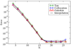
In general, optimality is difficult to check because both $uexact$ and its interpolant are unknown. However, for the test problem proposed in Section 2.5.2 this can be done. Figure 15 shows the maximum relative difference between the exact solution (64 ) and its interpolant and the various numerical solutions. All the curves behave in the same manner as $N$ increases, indicating that the three methods previously presented are optimal (at least for this particular case).

Figure 15: The difference between the exact solution (64

) of Equation (62

) and its interpolant (black curve) and between the exact and numerical solutions for i) the tau method (green curve and circle symbols) ii) the collocation method (blue curve and square symbols) iii) the Galerkin method (red curve and triangle symbols).