Spatial coordinate systems

3.1 Spatial coordinate systems

Most of the interesting problems in numerical relativity involve asymmetries that require the use of a full set of three-dimensional coordinates. We briefly review several coordinate sets (all orthogonal) that have been used in numerical relativity with spectral methods. They are described through the line element $ds2$ of the flat metric in the coordinates we discuss.

Cartesian (rectangular) coordinates are of course the simplest and most straightforward to implement; the line element reads $2 2 2 2 ds = dx + dy + dz$ . These coordinates are regular in all space, with vanishing connection, which makes them easy to use, since all differential operators have simple expressions and the associated triad is also perfectly regular. They are particularly well adapted to cube-like domains, see for instance [168 , 172 ] and [81 ] in the case of toroidal topology.
Circular cylindrical coordinates have a line element $ds2 = dρ2 + ρ2dϕ2 + dz2$ and exhibit a coordinate singularity on the $z$ -axis ( $ρ = 0$ ). The associated triad being also singular for $ρ = 0$ , regular vector or tensor fields have components that are multivalued (depending on $ϕ$ ) at any point of the $z$ -axis. As for the spherical coordinates, this can be handled quite easily with spectral methods. This coordinate system can be useful for axisymmetric or rotating systems, see [10 ].
Spherical (polar) coordinates will be discussed in more detail in Section 3.2. Their line element reads $ds2 = dr2 + r2d𝜃2 + r2sin2 𝜃dφ2$ , showing a coordinate singularity at the origin ( $r = 0$ ) and on the axis for which $𝜃 = 0,π$ . They are very useful in numerical relativity for the numerous sphere-like objects under study (stars, black hole horizons) and have mostly been implemented for shell-like domains [40 , 109 , 168 , 219 ] and for spheres including the origin [44 , 109 ].
Prolate spheroidal coordinates consist of a system of confocal ellipses and hyperbolae, describing an $(x, z)$ -plane, and an angle $φ$ giving the position as a rotation with respect to the focal axis [131 ]. The line element is $( ) ds2 = a2 sinh2 μ + sin2 ν (dμ2 + dν2) + a2 sinh2 μ sin2 νdφ2$ . The foci are situated at $z = ±a$ and represent coordinate singularities for $μ = 0$ and $ν = 0,π$ . These coordinates have been used in [8 ] with black-hole–puncture data at the foci.
Bispherical coordinates are obtained by the rotation of bipolar coordinates around the focal axis, with a line element $2 2 −2( 2 2 2 2) ds = a (cosh η − cosχ ) dη + dχ + sin χd φ$ . As with prolate spheroidal coordinates, the foci situated at $z = ±a$ ( $η → ±∞, χ = 0,π$ ) and more generally, the focal axis, exhibit coordinate singularities. Still, the surfaces of constant $η$ are spheres situated in the $z > 0(< 0)$ region for $η > 0(< 0)$ , respectively. Thus, these coordinates are very well adapted for the study of binary systems and in particular for excision treatment of black hole binaries [6 ].

3.1.1 Mappings

Choosing a smart set of coordinates is not the end of the story. As for finite elements, one would like to be able to cover some complicated geometries, like distorted stars, tori, etc…or even to be able to cover the whole space. The reason for this last point is that, in numerical relativity, one often deals with isolated systems for which boundary conditions are only known at spatial infinity. A quite simple choice is to perform a mapping from numerical coordinates to physical coordinates, generalizing the change of coordinates to $[− 1,1 ]$ , when using families of orthonormal polynomials or to $[0,2π]$ for Fourier series.

Figure 17: Regular deformation of the $[− 1,1] × [− 1,1]$ square.

An example of how to map the $[− 1,1] × [− 1,1]$ domain can be taken from Canuto et al. [56 ], and is illustrated in Figure 17 : once the mappings from the four sides (boundaries) of $ˆΩ$ to the four sides of $Ω$ are known, one can construct a two-dimensional regular mapping $Π$ , which preserves orthogonality and simple operators (see Chapter 3.5 of [56 ]).

The case where the boundaries of the considered domain are not known at the beginning of the computation can also be treated in a spectral way. In the case where this surface corresponds to the surface of a neutron star, two approaches have been used. First, in Bonazzola et al. [38 ], the star (and therefore the domain) is supposed to be “star-like”, meaning that there exists a point from which it is possible to reach any point on the surface by straight lines that are all contained inside the star. To such a point is associated the origin of a spherical system of coordinates, so that it is a spherical domain, which is regularly deformed to coincide with the shape of the star. This is done within an iterative scheme, at every step, once the position of the surface has been determined. Then, another approach has been developed by Ansorg et al. [10 ] using cylindrical coordinates. It is a square in the plane $(ρ,z)$ , which is mapped onto the domain describing the interior of the star. This mapping involves an unknown function, which is itself decomposed in terms of a basis of Chebyshev polynomials, so that its coefficients are part of the global vector of unknowns (as the density and gravitational field coefficients).

In the case of black-hole–binary systems, Scheel et al. [189 ] have developed horizon-tracking coordinates using results from control theory. They define a control parameter as the relative drift of the black hole position, and they design a feedback control system with the requirement that the adjustment they make on the coordinates be sufficiently smooth that they do not spoil the overall Einstein solver. In addition, they use a dual-coordinate approach, so that they can construct a comoving coordinate map, which tracks both orbital and radial motion of the black holes and allows them to successfully evolve the binary. The evolutions simulated in [189 ] are found to be unstable, when using a single rotating-coordinate frame. We note here as well the work of Bonazzola et al. [42 ], where another option is explored: the stroboscopic technique of matching between an inner rotating domain and an outer inertial one.

3.1.2 Spatial compactification

As stated above, the mappings can also be used to include spatial infinity into the computational domain. Such a compactification technique is not tied to spectral methods and has already been used with finite-difference methods in numerical relativity by, e.g., Pretorius [177 ]. However, due to the relatively low number of degrees of freedom necessary to describe a spatial domain within spectral methods, it is easier within this framework to use some resources to describe spatial infinity and its neighborhood. Many choices are possible to do so, either directly choosing a family of well-behaved functions on an unbounded interval, for example the Hermite functions (see, e.g., Section 17.4 in Boyd [48 ]), or making use of standard polynomial families, but with an adapted mapping. A first example within numerical relativity was given by Bonazzola et al. [41 ] with the simple inverse mapping in spherical coordinates.

This inverse mapping for spherical “shells” has also been used by Kidder and Finn [125

], Pfeiffer et al. [172

, 168

], and Ansorg et al. in cylindrical [10

] and spheroidal [8

] coordinates. Many more elaborated techniques are discussed in Chapter 17 of Boyd [48

], but to our knowledge, none have been used in numerical relativity yet. Finally, it is important to point out that, in general, the simple compactification of spatial infinity is not well adapted to solving hyperbolic PDEs and the above mentioned examples were solving only for elliptic equations (initial data, see Section 5). For instance, the simple wave equation (127

) is not invariant under the mapping (89

), as has been shown, e.g., by Sommerfeld (see [202

], Section 23.E). Intuitively, it is easy to see that when compactifying only spatial coordinates for a wave-like equation, the distance between two neighboring grid points becomes larger than the wavelength, which makes the wave poorly resolved after a finite time of propagation on the numerical grid. For hyperbolic equations, is is therefore usually preferable to impose physically and mathematically well-motivated boundary conditions at a finite radius (see, e.g., Friedrich and Nagy [83 ], Rinne [180

] or Buchman and Sarbach [53

]).

3.1.3 Patching in more than one dimension

The multidomain (or multipatch) technique has been presented in Section 2.6 for one spatial dimension. In Bonazzola et al. [40 ] and Grandclément et al. [109 ], the three-dimensional spatial domains consist of spheres (or star-shaped regions) and spherical shells, across which the solution can be matched as in one-dimensional problems (only through the radial dependence). In general, when performing a matching in two or three spatial dimensions, the reconstruction of the global solution across all domains might need some more care to clearly write down the matching conditions (see, e.g., [168 ], where overlapping as well as nonoverlapping domains are used at the same time). For example in two dimensions, one of the problems that might arise is the counting of matching conditions for corners of rectangular domains, when such a corner is shared among more than three domains. In the case of a PDE where matching conditions must be imposed on the value of the solution, as well as on its normal derivative (Poisson or wave equation), it is sufficient to impose continuity of either normal derivative at the corner, the jump in the other normal derivative being spectrally small (see Chapter 13 of Canuto et al. [56 ]).

Figure 18: Two sets of spherical domains describing a neutron star or black hole binary system. Each set is surrounded by a compactified domain of the type (89

), which is not displayed

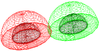
A now typical problem in numerical relativity is the study of binary systems (see also Sections 5.5 and 6.3) for which two sets of spherical shells have been used by Gourgoulhon et al. [100 ], as displayed in Figure 18 . Different approaches have been proposed by Kidder et al. [128 ], and used by Pfeiffer [168 ] and Scheel et al. [189 ] where spherical shells and rectangular boxes are combined together to form a grid adapted to black hole binary study. Even more sophisticated setups to model fluid flows in complicated tubes can be found in [144 ].

Multiple domains can thus be used to adapt the numerical grid to the interesting part (manifold) of the coordinate space; they can be seen as a technique close to the spectral element method [167 ]. Moreover, it is also a way to increase spatial resolution in some parts of the computational domain where one expects strong gradients to occur: adding a small domain with many degrees of freedom is the analog of fixed-mesh refinement for finite-differences.