Usual polynomials

2.4 Usual polynomials

2.4.1 Sturm–Liouville problems and convergence

The Sturm–Liouville problems are eigenvalue problems of the form:

on the interval $[− 1,1]$ . $p$ , $q$ and $w$ are real-valued functions such that:

$p(x)$ is continuously differentiable, strictly positive and continuous at $x = ±1$ .
$q(x)$ is continuous, non-negative and bounded.
$w (x)$ is continuous, non-negative and integrable.

The solutions are then the eigenvalues $λi$ and the eigenfunctions $ui (x)$ . The eigenfunctions are orthogonal with respect to the measure $w$ :

Singular Sturm–Liouville problems are particularly important for spectral methods. A Sturm–Liouville problem is singular if and only if the function $p$ vanishes at the boundaries $x = ±1$ . One can show, that if the functions of the spectral basis are chosen to be the solutions of a singular Sturm–Liouville problem, then the convergence of the function to its interpolant is faster than any power law of $N$ , $N$ being the order of the expansion (see Section 5.2 of [57 ]). One talks about spectral convergence. Let us be precise in saying that this does not necessarily imply that the convergence is exponential. Convergence properties are discussed in more detail for Legendre and Chebyshev polynomials in Section 2.4.4.

Conversely, it can be shown that spectral convergence is not ensured when considering solutions of regular Sturm–Liouville problems [57 ].

In what follows, two usual types of solutions of singular Sturm–Liouville problems are considered: Legendre and Chebyshev polynomials.

2.4.2 Legendre polynomials

Legendre polynomials $Pn$ are eigenfunctions of the following singular Sturm–Liouville problem:

In the notations of Equation (36

), $p = 1 − x2$ , $q = 0$ , $w = 1$ and $λn = − n(n + 1)$ .

It follows that Legendre polynomials are orthogonal on $[− 1,1]$ with respect to the measure $w (x) = 1$ . Moreover, the scalar product of two polynomials is given by:

Starting from $P = 1 0$ and $P = x 1$ , the successive polynomials can be computed by the following recurrence expression:

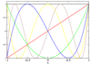
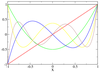
Among the various properties of Legendre polynomials, one can note that i) $P n$ has the same parity as $n$ . ii) $Pn$ is of degree $n$ . iii) $n Pn (±1 ) = (±1 )$ . iv) $Pn$ has exactly $n$ zeros on $[− 1,1]$ . The first polynomials are shown in Figure 8 .

Figure 8: First Legendre polynomials, from $P 0$ to $P 5$ .

The weights and locations of the collocation points associated with Legendre polynomials depend on the choice of quadrature.

Legendre–Gauss: $xi$ are the nodes of $PN+1$ and $wi = --------[-2--------]- (1 − x2i) P ′N+1 (xi)2$ .
Legendre–Gauss–Radau: $x = − 1 0$ and $x i$ are the nodes of $P + P N N+1$ . The weights are given by $2 w0 = -------2- (N + 1)$ and $1 wi = --------2 (N + 1)$ .
Legendre–Gauss–Lobatto: $x0 = − 1$ , $xN = 1$ and $xi$ are the nodes of $P ′N$ . The weights are $2 1 wi = -------------------2- N (N + 1) [PN (xi)]$ .

These values have no analytic expression, but they can be computed numerically in an efficient way.

Some elementary operations can easily be performed on the coefficient space. Let us assume that a function $f$ is given by its coefficients $an$ so that $N ∑ f = anPn n=0$ . Then, the coefficients $bn$ of $∑N Hf = bnPn n=0$ can be found as a function of $an$ , for various operators $H$ . For instance,

if $H$ is multiplication by $x$ then:
if $H$ is the derivative:
if $H$ is the second derivative:

These kind of relations enable one to represent the action of $H$ as a matrix acting on the vector of $an$ , the product being the coefficients of $Hf$ , i.e. the $bn$ .

2.4.3 Chebyshev polynomials

Chebyshev polynomials $Tn$ are eigenfunctions of the following singular Sturm–Liouville problem:

In the notation of Equation (36

), $√ ------- p = 1 − x2$ , $q = 0$ , $√ ------- w = 1∕ 1 − x2$ and $λn = − n$ .

It follows that Chebyshev polynomials are orthogonal on $[− 1, 1]$ with respect to the measure $w = 1∕√1--−-x2-$ and the scalar product of two polynomials is

Given that $T0 = 1$ and $T1 = x$ , the higher-order polynomials can be obtained by making use of the recurrence

This implies the following simple properties: i) $Tn$ has the same parity as $n$ ; ii) $Tn$ is of degree $n$ ; iii) $Tn(±1 ) = (±1 )n$ ; iv) $Tn$ has exactly $n$ zeros on $[− 1,1 ]$ . The first polynomials are shown in Figure 9

Figure 9: First Chebyshev polynomials, from $T 0$ to $T 5$ .

Contrary to the Legendre case, both the weights and positions of the collocation points are given by analytic formulae:

Chebyshev–Gauss: $x = cos (2i-+-1)π i 2N + 2$ and $w = --π--- i N + 1$ .
Chebyshev–Gauss–Radau: $2πi xi = cos-------- 2N + 1$ . The weights are $π w0 = -------- 2N + 1$ and $wi = ---2π--- 2N + 1$ .
Chebyshev–Gauss–Lobatto: $πi xi = cos--- N$ . The weights are $π w0 = wN = ---- 2N$ and $π wi = --- N$ .

As for the Legendre case, the action of various linear operators $H$ can be expressed in the coefficient space. This means that the coefficients $bn$ of $Hf$ are given as functions of the coefficients $an$ of $f$ . For instance,

if $H$ is multiplication by $x$ :
if $H$ is the derivative:
if $H$ is the second derivative:

2.4.4 Convergence properties

One of the main advantages of spectral methods is the very fast convergence of the interpolant $INf$ to the function $f$ , at least for smooth enough functions. Let us consider a $𝒞m$ function $f$ ; one can place the following upper bounds on the difference between $f$ and its interpolant $IN f$ :

For Legendre:
For Chebyshev:

The $Ci$ are positive constants. An interesting limit of the above estimates concerns a $𝒞∞$ function. One can then see that the difference between $f$ and $I f N$ decays faster than any power of $N$ . This is spectral convergence. Let us be precise in saying that this does not necessarily imply that the error decays exponentially (think about $( √ --) exp − N$ , for instance). Exponential convergence is achieved only for analytic functions, i.e. functions that are locally given by a convergent power series.

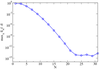
An example of this very fast convergence is shown in Figure 10 . The error clearly decays exponentially, the function being analytic, until it reaches the level of machine precision, 10^–14 (one is working in double precision in this particular case). Figure 10 illustrates the fact that, with spectral methods, very good accuracy can be reached with only a moderate number of coefficients.

Figure 10: Maximum difference between $f = cos3 (πx∕2) + (x + 1)3∕8$ and its interpolant $I f N$ , as a function of $N$ .

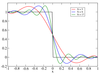
If the function is less regular (i.e. not $∞ 𝒞$ ), the error only decays as a power law, thus making the use of spectral method less appealing. It can easily be seen in the worst possible case: that of a discontinuous function. In this case, the estimates (50 -52 ) do not even ensure convergence. Figure 11 shows a step function and its interpolant for various values of $N$ . One can see that the maximum difference between the function and its interpolant does not go to zero even when $N$ is increasing. This is known as the Gibbs phenomenon.

Finally, Equation (52 ) shows that, if $m > 0$ , the interpolant converges uniformly to the function. Continuous functions that do not converge uniformly to their interpolant, whose existence has been shown by Faber [73 ] (see Section 2.2), must belong to the $𝒞0$ functions. Indeed, for the case $m = 0$ , Equation (52 ) does not prove convergence (neither do Equations (50 ) or (51 )).

Figure 11: Step function (black curve) and its interpolant, for various values of $N$ .

2.4.5 Trigonometric functions

A detailed presentation of the theory of Fourier transforms is beyond the scope of this work. However, there is a close link between discrete Fourier transforms and their spectral interpolation, which is briefly outlined here. More detail can be found, for instance, in [57 ].

The Fourier transform $P f$ of a function $f$ of $[0,2π ]$ is given by:

The Fourier transform is known to converge rather rapidly to the function itself, if $f$ is periodic. However, the coefficients $an$ and $bn$ are given by integrals of the form $∫ 2π f (x) cos(nx )dx 0$ , that cannot easily be computed (as was the case for the projection of a function on orthogonal polynomials in Section 2.3.1).

The solution to this problem is also very similar to the use of the Gaussian quadratures. Let us introduce $N + 1$ collocation points $xi = 2πi∕(N + 1)$ . Then the discrete Fourier coefficients with respect to those points are:

1 ∑N &tidle;a0 = --- f (xk) , (54 ) N k=1 N -2-∑ &tidle;an = N f (xk) cos(nxk) , (55 ) k=1 2 ∑N &tidle;bn = --- f (xk) sin (nxk) (56 ) N k=1

and the interpolant $INf$ is then given by:

The approximation made by using discrete coefficients in place of real ones is of the same nature as the one made when computing coefficients of projection (30 ) by means of the Gaussian quadratures. Let us mention that, in the case of a discrete Fourier transform, the first and last collocation points lie on the boundaries of the interval, as for a Gauss-Lobatto quadrature. As for the polynomial interpolation, the convergence of $INf$ to $f$ is spectral for all periodic and $𝒞∞$ functions.

2.4.6 Choice of basis

For periodic functions of $[0,2π[$ , the discrete Fourier transform is the natural choice of basis. If the considered function has also some symmetries, one can use a subset of the trigonometric polynomials. For instance, if the function is i) periodic on $[0,2π [$ and is also odd with respect to $x = π$ , then it can be expanded in terms of sines only. If the function is not periodic, then it is natural to expand it either in Chebyshev or Legendre polynomials. Using Legendre polynomials can be motivated by the fact that the associated measure is very simple: $w (x) = 1$ . The multidomain technique presented in Section 2.6.5 is one particular example in which such a property is required. In practice, Legendre and Chebyshev polynomials usually give very similar results.