Time discretization

4.1 Time discretization

There have been very few theoretical developments in spectral time discretization, with the exception of Ierley et al. [121

], where the authors have applied spectral methods in time to the study of the Korteweg–de Vries and Burger equations, using Fourier series in space and Chebyshev polynomials for the time coordinates. Ierley et al. [121 ] observe a timestepping restriction: they have to employ multidomain and patching techniques (see Section 2.6) for the time interval, with the size of each subdomain being roughly given by the Courant–Friedrichs–Lewy (CFL) condition. Therefore, the most common approach for time representation are finite-difference techniques, which allow for the use of many well-established time-marching schemes, and the method of lines (for other methods, including fractional stepping, see Fornberg [79 ]). Let us write the general form of a first-order-in-time linear PDE:

where $L$ is a linear operator containing only derivatives with respect to the spatial coordinate $x$ . For every value of time $t$ , the spectral approximation $uN (x,t)$ is a function of only one spatial dimension belonging to some finite-dimensional subspace of the suitable Hilbert space $ℋ$ , with the given $L2 w$ spatial norm, associated for example with the scalar product and the weight $w$ introduced in Section 2.3.1. Formally, the solution of Equation (116

) can be written as:

In practice, to integrate time-dependent problems one can use spectral methods to calculate spatial derivatives and standard finite-difference schemes to advance in time.

4.1.1 Method of lines

At every instant $t$ , one can represent the function $uN(x, t)$ by a finite set $UN (t)$ , composed of its time-dependent spectral coefficients or its values at the collocation points. We denote $LN$ the spectral approximation to the operator $L$ , together with the boundary conditions, if the tau or collocation method is used. $L N$ is, therefore, represented as an $N × N$ matrix. This is the method of lines, which allows one to reduce a PDE to an ODE, after discretization in all but one dimensions. The advantage is that many ODE integration schemes are known (Runge–Kutta, symplectic integrators, ...) and can be used here. We shall suppose an equally-spaced grid in time, with the timestep noted $Δt$ and $U J = UN (J × Δt ) N$ .

In order to step from $J U N$ to $J+1 UN$ , one has essentially two possibilities: explicit and implicit schemes. In an explicit scheme, the action of the spatial operator $LN$ on $K || U N K≤J$ must be computed to explicitly get the new values of the field (either spatial spectral coefficients or values at collocation points). A simple example is the forward Euler method:

which is first order and for which, as for any explicit schemes, the timestep is limited by the CFL condition. The imposition of boundary conditions is discussed in Section 4.2. With an implicit scheme one must solve for a boundary value problem in term of $U J+1 N$ at each timestep: it can be performed in the same way as for the solution of the elliptic equation (62

) presented in Section 2.5.2. The simplest example is the backward Euler method:

which can be re-written as an equation for the unknown $J+1 U N$ :

J+1 J (I + ΔtLN ) UN = UN ,

where $I$ is the identity operator. Both schemes have different stability properties, which can be analyzed as follows. Assuming that $L N$ can be diagonalized in the sense of the definition given in (4.1.3), the stability study can be reduced to the study of the collection of scalar ODE problems

where $λi$ is any of the eigenvalues of $LN$ in the sense of Equation (124

4.1.2 Stability

The basic definition of stability for an ODE integration scheme is that, if the timestep is lower than some threshold, then $∥U J∥ ≤ AeKJ Δt N$ , with constants $A$ and $K$ independent of the timestep. This is perhaps not the most appropriate definition, since in practice one often deals with bounded functions and an exponential growth in time would not be acceptable. Therefore, an integration scheme is said to be absolutely stable (or asymptotically stable), if $∥U JN ∥$ remains bounded, $∀J ≥ 0$ . This property depends on a particular value of the product $λi × Δt$ . For each time integration scheme, the region of absolute stability is the set of the complex plane containing all the $λ Δt i$ for which the scheme is absolutely stable.

Figure 20: Regions of absolute stability for the Adams–Bashforth integration schemes of order one to four.

Finally, a scheme is said to be $A$ -stable if its region of absolute stability contains the half complex plane of numbers with negative real part. It is clear that no explicit scheme can be $A$ -stable due to the CFL condition. It has been shown by Dahlquist [66 ] that there is no linear multistep method of order higher than two, which is $A$ -stable. Thus implicit methods are also limited in timestep size, if more than second-order accurate. In addition, Dahlquist [66 ] shows that the most accurate second-order $A$ -stable scheme is the trapezoidal one (also called Crank–Nicolson, or second-order Adams–Moulton scheme)

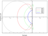
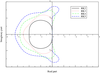
Figure 21: Regions of absolute stability for the Runge–Kutta integration schemes of order two to five. Note that the size of the region increases with order.

Figures 20 and 21 display the absolute stability regions for the Adams–Bashforth and Runge–Kutta families of explicit schemes (see, for instance, [56 ]). For a given type of spatial linear operator, the requirement on the timestep usually comes from the largest (in modulus) eigenvalue of the operator. For example, in the case of the advection equation on $[− 1,1]$ , with a Dirichlet boundary condition,

and using a Chebyshev-tau method, one can see that the largest eigenvalue of $LN$ grows in modulus as $2 N$ . Therefore, for any of the schemes considered in Figures 20

and 21

, the timestep has a restriction of the type

which can be related to the usual CFL condition by the fact that the minimal distance between two points of a ( $N$ -point) Chebyshev grid decreases like $O (N −2)$ . Due to the above mentioned Second Dahlquist barrier [66 ], implicit time marching schemes of order higher than two also have such a limitation.

4.1.3 Spectrum of simple spatial operators

An important issue in determining the absolute stability of a time-marching scheme for the solution of a given PDE is the computation of the spectrum $(λi)$ of the discretized spatial operator $LN$ (120 ). As a matter of fact, these eigenvalues are those of the matrix representation of $LN$ , together with the necessary boundary conditions for the problem to be well posed (e.g., $ℬN u = 0$ ). If one denotes $b$ the number of such boundary conditions, each eigenvalue $λi$ (here, in the case of the tau method) is defined by the existence of a non-null set of coefficients ${cj}1≤j≤N$ such that

Figure 22: Eigenvalues of the first derivative-tau operator (124

) for Chebyshev polynomials. The largest (in modulus) eigenvalue is not displayed; this one is real, negative and goes as $O(N 2)$ .

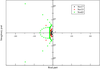
As an example, let us consider the case of the advection equation (first-order spatial derivative) with a Dirichlet boundary condition, solved with the Chebyshev-tau method (122 ). Because of the definition of the problem (124 ), there are $N − 1$ “eigenvalues”, which can be computed, after a small transformation, using any standard linear algebra package. For instance, it is possible, making use of the boundary condition, to express the last coefficient as a combination of the other ones

One is thus left with the usual eigenvalue problem for an $(N − 1) × (N − 1)$ matrix. Results are displayed in Figure 22

for three values of $N$ . Real parts are all negative: the eigenvalue that is not displayed lies on the negative part of the real axis and is much larger in modulus (it is growing as $2 O (N )$ ) than the $N − 1$ others.

This way of determining the spectrum can be, of course, generalized to any linear spatial operator, for any spectral basis, as well as to the collocation and Galerkin methods. Intuitively from CFL-type limitations, one can see that in the case of the heat equation ( $Lu = ∂2u∕∂x2$ ), explicit time-integration schemes (or any scheme that is not $A$ -stable) will have a severe timestep limitation of the type

for both a Chebyshev or Legendre decomposition basis. Finally, one can decompose a higher-order-in-time PDE into a first-order system and then use one of the above proposed schemes. In the particular case of the wave equation,

it is possible to write a second-order Crank-Nicolson scheme directly [158

Since this scheme is $A$ -stable, there is no limitation on the timestep $Δt$ , but for explicit or higher-order schemes this limitation would be $−2 Δt ≲ O(N )$ , as for the advection equation. The solution of such an implicit scheme is obtained as that of a boundary value problem at each timestep.

4.1.4 Semi-implicit schemes

It is sometimes possible to use a combination of implicit and explicit schemes to loosen a timestep restriction of the type (123 ). Let us consider, as an example, the advection equation with nonconstant velocity on $[− 1,1]$ ,

with the relevant boundary conditions, which shall in general depend on the sign of $v(x)$ . If, on the one hand, the stability condition for explicit time schemes (123

) is too strong, and on the other hand an implicit scheme is too lengthy to implement or to use (because of the nonconstant coefficient $v(x )$ ), then it is interesting to consider the semi-implicit two-step method (see also [94

])

U J+1∕2− Δt-L− UJ+1 ∕2 = U J + Δt- (L − L− )U J, N 2 N N N 2 N N N J+1 Δt + J+1 J+1∕2 Δt ( +) J+1∕2 U N − ---L NU N = U N + --- LN − L N UN , (130 ) 2 2

where $+ LN$ and $− L N$ are respectively the spectral approximations to the constant operators $− v(1)∂∕∂x$ and $− v (− 1)∂∕ ∂x$ , together with the relevant boundary conditions (if any). This scheme is absolutely stable if

With this type of scheme, the propagation of the wave at the boundary of the interval is treated implicitly, whereas the scheme is still explicit in the interior. The implementation of the implicit part, for which one needs to solve a boundary-value problem, is much easier than for the initial operator (129

) because of the presence of only constant-coefficient operators. This technique is quite helpful in the case of more severe timestep restrictions (126

), for example for a variable coefficient heat equation.