Multidomain techniques for ODEs

2.6 Multidomain techniques for ODEs

2.6.1 Motivations and setting

As seen in Section 2.4.4, spectral methods are very efficient when dealing with $𝒞∞$ functions. However, they lose some of their appeal when dealing with less regular functions, the convergence to the exact functions being substantially slower. Nevertheless, the physicist has sometimes to deal with such functions. This is the case for the density jump at the surface of strange stars or the formation of shocks, to mention only two examples. In order to maintain spectral convergence, one then needs to introduce several computational domains such that the various discontinuities of the functions lie at the interface between the domains. Doing so in each domain means that one only deals with $𝒞 ∞$ functions.

Multidomain techniques can also be valuable when dealing with a physical space either too complicated or too large to be described by a single domain. Related to that, one can also use several domains to increase the resolution in some parts of the space where more precision is required. This can easily be done by using a different number of basis functions in different domains. One then talks about fixed-mesh refinement.

Efficient parallel processing may also require that several domains be used. Indeed, one could set a solver, dealing with each domain on a given processor, and interprocessor communication would then only be used for matching the solution across the various domains. The algorithm of Section 2.6.4 is well adapted to such purposes.

In the following, four different multidomain methods are presented to solve an equation of the type $Lu = S$ on $[− 1,1]$ . $L$ is a second-order linear operator and $S$ is a given source function. Appropriate boundary conditions are given at the boundaries $x = − 1$ and $x = 1$ .

For simplicity the physical space is split into two domains:

first domain: $x ≤ 0$ described by $x1 = 2x + 1, x1 ∈ [− 1,1]$ ,
second domain: $x ≥ 0$ described by $x2 = 2x − 1, x2 ∈ [− 1,1]$ .

If $x ≤ 0$ , a function $u$ is described by its interpolant in terms of $x1$ : $N∑ IN u (x ) = &tidle;u1iTi (x1(x)) i=0$ . The same is true for $x ≥ 0$ with respect to the variable $x2$ . Such a set-up is obviously appropriate to deal with problems where discontinuities occur at $x = 0$ , that is $x1 = 1$ and $x2 = − 1$ .

2.6.2 The multidomain tau method

As for the standard tau method (see Section 2.5.2) and in each domain, the test functions are the basis polynomials and one writes the associated residual equations. For instance, in the domain $x ≤ 0$ one gets:

$1 &tidle;s$ being the coefficients of the source and $Lij$ the matrix representation of the operator. As for the one-domain case, one relaxes the last two equations, keeping only $N − 1$ equations. The same is done in the second domain.

Two supplementary equations are enforced to ensure that the boundary conditions are fulfilled. Finally, the operator $L$ being of second order, one needs to ensure that the solution and its first derivative are continuous at the interface $x = 0$ . This translates to a set of two additional equations involving both domains.

So, one considers

$N − 1$ residual equations in the first domain,
$N − 1$ residual equations in the second domain,
2 boundary conditions,
2 matching conditions,

for a total of $2N + 2$ equations. The unknowns are the coefficients of $u$ in both domains (i.e. the $1 &tidle;ui$ and the $&tidle;u2i$ ), that is $2N + 2$ unknowns. The system is well posed and admits a unique solution.

2.6.3 Multidomain collocation method

As for the standard collocation method (see Section 2.5.3) and in each domain, the test functions are the Lagrange cardinal polynomials. For instance, in the domain $x ≤ 0$ one gets:

$Lij$ being the matrix representation of the operator and $x1n$ the $nth$ collocation point in the first domain. As for the one-domain case, one relaxes the two equations corresponding to the boundaries of the domain, keeping only $N − 1$ equations. The same is done in the second domain.

Two supplementary equations are enforced to ensure that the boundary conditions are fulfilled. Finally, the operator $L$ being second order, one needs to ensure that the solution and its first derivative are continuous at the interface $x = 0$ . This translates to a set of two additional equations involving the coefficients in both domains.

So, one considers

$N − 1$ residual equations in the first domain,
$N − 1$ residual equations in the second domain,
2 boundary conditions,
2 matching conditions,

for a total of $2N + 2$ equations. The unknowns are the coefficients of $u$ in both domains (i.e. the $&tidle;u1i$ and the $&tidle;u2i$ ), that is $2N + 2$ unknowns. The system is well posed and admits a unique solution.

2.6.4 Method based on homogeneous solutions

The method described here proceeds in two steps. First, particular solutions are computed in each domain. Then, appropriate linear combinations with the homogeneous solutions of the operator $L$ are performed to ensure continuity and impose boundary conditions.

In order to compute particular solutions, one can rely on any of the methods described in Section 2.5. The boundary conditions at the boundary of each domain can be chosen (almost) arbitrarily. For instance, one can use in each domain a collocation method to solve $Lu = S$ , demanding that the particular solution $upart$ is zero at both ends of each interval.

Then, in order to have a solution over the whole space, one needs to add homogeneous solutions to the particular ones. In general, the operator $L$ is second order and admits two independent homogeneous solutions $g$ and $h$ in each domain. Let us note that, in some cases, additional regularity conditions can reduce the number of available homogeneous solutions. The homogeneous solutions can either be computed analytically if the operator $L$ is simple enough or numerically, but one must then have a method for solving $Lu = 0$ .

In each domain, the physical solution is a combination of the particular solution and homogeneous ones of the type:

where $α$ and $β$ are constants that must be determined. In the two domains case, we are left with four unknowns. The system of equations they must satisfy is composed of i) two equations for the boundary conditions ii) two equations for the matching of $u$ and its first derivative across the boundary between the two domains. The obtained system is called the matching system and generally admits a unique solution.

2.6.5 Variational method

Contrary to previously presented methods, the variational one is only applicable with Legendre polynomials. Indeed, the method requires that the measure be $w (x) = 1$ . It is also useful to extract the second-order term of the operator $L$ and to rewrite it as $Lu = u ′′ + H$ , $H$ being first order only.

In each domain, one writes the residual equation explicitly:

The term involving the second derivative of $u$ is then integrated by parts:

The test functions are the same as the ones used for the collocation method, i.e. functions being zero at all but one collocation point, in both domains ( $d = 1,2$ ): $ξi(xdj) = δij$ . By making use of the Gauss quadratures, the various parts of Equation (79 ) can be expressed as ( $d = 1,2$ indicates the domain):

∫ ′ ′ ∑N ′ ′ ∑N ∑N ξnu dx = ξn(xdi)u (xdi)wi = DijDinwiu (xdj), (80 ) i=0 i=0 j=0 ∫ ∑N ∑N ξ (Hu ) dx = ξ (x )(Hu )(x )w = w H u(x ), (81 ) n n di di i n ni di ∫ i=0 i=0 ∑N ξnSdx = ξn(xdi)S (xdi)wi = S (xdn)wn, (82 ) i=0

where $D ij$ (or $H ij$ , respectively) represents the action of the derivative (or of $H$ , respectively) in the configuration space

∑N g′(xdk) = Dkjg (xdj) , (83 ) j=0 ∑N (Hg )(xdk) = Hkjg (xdj) . (84 ) j=0

For points strictly inside each domain, the integrated term $[ξu ′]$ of Equation (79 ) vanishes and one gets equations of the form:

This is a set of $N − 1$ equations for each domains ( $d = 1, 2$ ). In the above form, the unknowns are the $u (x ) di$ , i.e. the solution is sought in the configuration space.

As usual, two additional equations are provided by appropriate boundary conditions at both ends of the global domain. One also gets an additional condition by matching the solution across the boundary between the two domains.

The last equation of the system is the matching of the first derivative of the solution. However, instead of writing it “explicitly”, this is done by making use of the integrated term in Equation (79 ) and this is actually the crucial step of the whole method. Applying Equation (79 ) to the last point $x1N$ of the first domain, one gets:

The same can be done with the first point of the second domain to get $′ u (x2 = − 1)$ , and the last equation of the system is obtained by demanding that $u′(x1 = 1) = u′(x2 = − 1)$ and relates the values of $u$ in both domains.

Before finishing with the variational method, it may be worthwhile to explain why Legendre polynomials are used. Suppose one wants to work with Chebyshev polynomials instead. The measure is then $---1---- w (x ) = √1-−--x2-$ . When one integrates the term containing $′′ u$ by parts, one gets

Because the measure is divergent at the boundaries, it is difficult, if not impossible, to isolate the term in $u ′$ . On the other hand, this is precisely the term that is needed to impose the appropriate matching of the solution.

2.6.6 Merits of the various methods

From a numerical point of view, the method based on an explicit matching using the homogeneous solutions is somewhat different from the two others. Indeed, one must solve several systems in a row and each one is of the same size as the number of points in one domain. This splitting of the different domains can also be useful for designing parallel codes. On the contrary, for both the variational and the tau method one must solve only one system, but its size is the same as the number of points in a whole space, which can be quite large for many domains settings. However, those two methods do not require one to compute the homogeneous solutions, computation that could be tricky depending on the operators involved and the number of dimensions.

The variational method may seem more difficult to implement and is only applicable with Legendre polynomials. However, on mathematical grounds, it is the only method that is demonstrated to be optimal. Moreover, some examples have been found in which the others methods are not optimal. It remains true that the variational method is very dependent on both the shape of the domains and the type of equation that needs to be solved.

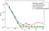
The choice of one method or another thus depends on the particular situation. As for the mono-domain space, for simple test problems the results are very similar. Figure 16 shows the maximum error between the analytic solution and the numeric one for the four different methods. All errors decay exponentially and reach machine accuracy within roughly the same number of points.

Figure 16: Difference between the exact and numerical solutions of the following test problem. $2 d-u-+ 4u = S dx2$ , with $S (x < 0 ) = 1$ and $S (x > 0) = 0$ . The boundary conditions are $u (x = − 1) = 0$ and $u (x = 1) = 0$ . The black curve and circles denote results from the multidomain tau method, the red curve and squares from the method based on the homogeneous solutions, the blue curve and diamonds from the variational one, and the green curve and triangles from the collocation method.