Imposition of boundary conditions

4.2 Imposition of boundary conditions

The time-dependent PDE (116

) can be written as a system of ODEs in time either for the time-dependent spectral coefficients ${ci(t)}i=0...N$ of the unknown function $u (x,t)$ (Galerkin or tau methods), or for the time-dependent values at collocation points ${u(xi,t)} i=0...N$ (collocation method). Implicit time-marching schemes (like the backward Euler scheme (119

)) are technically very similar to a succession of boundary-value problems, as for elliptic equations or Equation (62

) described in Section 2.5. The coefficients (or the values at collocation points) are determined at each new timestep by inversion of the matrix of type $I + ΔtL$ or its higher-order generalization. To represent a well-posed problem, this matrix needs, in general, the incorporation of boundary conditions, for tau and collocation methods. Galerkin methods are not so useful if the boundary conditions are time dependent: this would require the construction of a new Galerkin basis at each new timestep, which is too complicated and/or time consuming. We shall therefore discuss in the following sections the imposition of boundary conditions for explicit time schemes, with the tau or collocation methods.

4.2.1 Strong enforcement

The standard technique is to enforce the boundary conditions exactly, i.e. up to machine precision. Let us suppose here that the time-dependent PDE (116 ), which we want to solve, is well posed with boundary condition

where $b(t)$ is a given function. We give here some examples, with the forward Euler scheme (118

) for time discretization.

In the collocation method, the values of the approximate solution at (Gauss–Lobatto type) collocation points ${xi}i=0...N$ are determined by a system of equations:

where the value at the boundary $(x = 1)$ is directly set to be the boundary condition.

In the tau method, the vector $U J N$ is composed of the $N + 1$ coefficients ${c (J × Δt )} i i=0...N$ at the $J$ -th timestep. If we denote by $( J) LN UN i$ the $i$ -th coefficient of $LN$ applied to $J U N$ , then the vector of coefficients ${ci}i=0...N$ is advanced in time through the system:

( J) ∀i = 0 ...N − 1, ci((J + 1) × Δt ) = ci(J × Δt) + Δt LN U N i (134 ) N∑−1 cN ((J + 1) × Δt ) = b((J + 1)Δt ) − ck, k=0

the last equality ensures the boundary condition in the coefficient space.

4.2.2 Penalty approach

As shown in the previous examples, the standard technique consists of neglecting the solution to the PDE for one degree of freedom, in configuration or coefficient space, and using this degree of freedom in order to impose the boundary condition. However, it is interesting to try and impose a linear combination of both the PDE and the boundary condition on this last degree of freedom, as is shown by the next simple example. We consider the simple (time-independent) integration over the interval $x ∈ [− 1, 1]$ :

where $u(x)$ is the unknown function. Using a standard Chebyshev relation (161

)collocation method (see Section 2.5.3), we look for an approximate solution $uN$ as a polynomial of degree $N$ verifying

duN-- ∀i = 0 ...N − 1, dx (xi) = sin (xi − 1), duN ----(xN = 1) = 0, dx

where ${xi}i=0...N$ are the Chebyshev–Gauss–Lobatto collocation points.

Figure 23: Behavior of the error in the solution of the differential equation (135

), as a function of the parameter $τ$ entering the numerical scheme (136

We now adopt another procedure that takes into account the differential equation at the boundary as well as the boundary condition, with $uN$ verifying (remember that $xN = 1$ ):

∀i = 0...N − 1, duN-(x ) = sin(x − 1), (136 ) dx i i duN -----(xN ) − τuN (xN ) = sin(xN − 1), dx

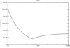
where $τ > 0$ is a constant; one notices when taking the limit $τ → + ∞$ , that both systems become equivalent. The discrepancy between the numerical and analytical solutions is displayed in Figure 23

, as a function of that parameter $τ$ , when using $N = 8$ . It is clear from that figure that there exists a finite value of $τ$ ( $τ ≃ 70 min$ ) for which the error is minimal and, in particular, lower than the error obtained by the standard technique. Numerical evidence indicates that $2 τmin ∼ N$ . This is a simple example of weakly imposed boundary conditions, with a penalty term added to the system. The idea of imposing boundary conditions up to the order of the numerical scheme was first proposed by Funaro and Gottlieb [85 ] and can be efficiently used for time-dependent problems, as illustrated by the following example. For a more detailed description, we refer the interested reader to the review article by Hesthaven [115

Let us consider the linear advection equation

where $f(t)$ is a given function. We look for a Legendre collocation method to obtain a solution, and define the polynomial $Q− (x)$ , which vanishes on the Legendre–Gauss–Lobatto grid points, except at the boundary $x = 1$ :

′ Q − (x) = (1-+-x)P-N(x) . 2P ′N (1 )

Thus, the Legendre collocation penalty method uniquely defines a polynomial $uN (x,t)$ through its values at Legendre–Gauss–Lobatto collocation points ${xi}i=0...N$

where $τ$ is a free parameter as in Equation (136

). For all the grid points, except the boundary one, this is the same as the standard Legendre collocation method ( $∀i = 0...N − 1, Q − (xi) = 0$ ). At the boundary point $x = xN = 1$ , one has a linear combination of the advection equation and the boundary condition. Contrary to the case of the simple integration (136

), the parameter $τ$ here cannot be too small: in the limit $τ → 0$ , the problem is ill posed and the numerical solution diverges. On the other hand, we still recover the standard (strong) imposition of boundary conditions when $τ → +∞$ . With the requirement that the approximation be asymptotically stable, we get for the discrete energy estimate (see the details of this technique in Section 4.3.2) the requirement

1 d ∑N ∂uN || ----∥uN (t)∥2 = uN (xi,t) ----|| wi − τu2N (t,xN)wN ≤ 0. 2 dt i=0 ∂x x=xi

Using the property of Gauss–Lobatto quadrature rule (with the Legendre–Gauss–Lobatto weights $wi$ ), and after an integration by parts, the stability is obtained if

It is also possible to treat more complex boundary conditions, as described in Hesthaven and Gottlieb [116 ] in the case of Robin-type boundary conditions (see Section 2.5.1 for a definition). Specific conditions for the penalty coefficient $τ$ are derived, but the technique is the same: for each boundary, a penalty term is added, which is proportional to the error on the boundary condition at the considered time. Thus, nonlinear boundary operators can also be incorporated easily (see, e.g., the case of the Burgers equation in [115 ]). The generalization to multidomain solutions is straightforward: each domain is considered as an isolated one, which requires boundary conditions at every timestep. The condition is imposed through the penalty term containing the difference between the junction conditions. This approach has very strong links with the variational method presented in Section 2.6.5 in the case of time-independent problems. A more detailed discussion of the weak imposition of boundary conditions is given in Canuto et al. (Section 3.7 of [57

] and Section 5.3 of [58 ] for multidomain methods).