2.2 Interpolation on a grid
A grid  on the interval
 ![[− 1,1]](article110x.gif) is a set of
is a set of  points
 ![xi ∈ [− 1, 1]](article112x.gif) ,
,  . These points
are called the nodes of the grid
. These points
are called the nodes of the grid  .
.
Let us consider a continuous function  and a family of grids
  with
with  nodes
nodes  . Then,
there exists a unique polynomial of degree
. Then,
there exists a unique polynomial of degree  ,
,  , that coincides with
  at each node:
 is called the interpolant of
  through the grid
  .
.  can be expressed in terms of the
Lagrange cardinal polynomials:
can be expressed in terms of the
Lagrange cardinal polynomials:
where  are the Lagrange cardinal polynomials. By definition,
  is the unique polynomial of degree
 that vanishes at all nodes of the grid
  , except at
  , where it is equal to one. It is easy to show
that the Lagrange cardinal polynomials can be written as
Figure 2 shows some examples of Lagrange cardinal polynomials. An example of a function and its
interpolant on a uniform grid can be seen in Figure 3.
, where it is equal to one. It is easy to show
that the Lagrange cardinal polynomials can be written as
Figure 2 shows some examples of Lagrange cardinal polynomials. An example of a function and its
interpolant on a uniform grid can be seen in Figure 3.
Thanks to Chebyshev alternate theorem, one can see that the best approximation of degree  is an
interpolant of the function at
is an
interpolant of the function at  nodes. However, in general, the associated grid is not known. The
difference between the error made by interpolating on a given grid
nodes. However, in general, the associated grid is not known. The
difference between the error made by interpolating on a given grid  can be compared to the
smallest possible error for the best approximation. One can show that (see Prop. 7.1 of [179
can be compared to the
smallest possible error for the best approximation. One can show that (see Prop. 7.1 of [179 ]):
]):
where  is the Lebesgue constant of the grid
  and is defined as:
A theorem by Erdös [72] states that, for any choice of grid  , there exists a constant
  such
that:
such
that:
It immediately follows that  when
when  . This is related to a result from 1914 by Faber [73]
that states that for any grid, there always exists at least one continuous function
. This is related to a result from 1914 by Faber [73]
that states that for any grid, there always exists at least one continuous function  , whose
interpolant does not converge uniformly to
, whose
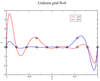
interpolant does not converge uniformly to  . An example of such failure of convergence is show in
Figure 4, where the convergence of the interpolant to the function
. An example of such failure of convergence is show in
Figure 4, where the convergence of the interpolant to the function  is clearly
nonuniform (see the behavior near the boundaries of the interval). This is known as the Runge
phenomenon.
is clearly
nonuniform (see the behavior near the boundaries of the interval). This is known as the Runge
phenomenon.
Moreover, a theorem by Cauchy (theorem 7.2 of [179]) states that, for all functions  , the
interpolation error on a grid
, the
interpolation error on a grid  of
of  nodes is given by
where ![𝜖 ∈ [− 1,1]](article162x.gif) .
.  is the nodal polynomial of
  , being the only polynomial of degree
  ,
with a leading coefficient of
,
with a leading coefficient of  , and that vanishes on the nodes of
  . It is then easy to show that
In Equation (25), one has a priori no control on the term involving  . For a given function, it can
be rather large and this is indeed the case for the function
. For a given function, it can
be rather large and this is indeed the case for the function  shown in Figure 4 (one can check, for
instance, that
shown in Figure 4 (one can check, for
instance, that  becomes larger and larger). However, one can hope to minimize the interpolation
error by choosing a grid such that the nodal polynomial is as small as possible. A theorem by Chebyshev
states that this choice is unique and is given by a grid, whose nodes are the zeros of the Chebyshev
polynomial
becomes larger and larger). However, one can hope to minimize the interpolation
error by choosing a grid such that the nodal polynomial is as small as possible. A theorem by Chebyshev
states that this choice is unique and is given by a grid, whose nodes are the zeros of the Chebyshev
polynomial  (see Section 2.3 for more details on Chebyshev polynomials). With such a grid, one can
achieve
(see Section 2.3 for more details on Chebyshev polynomials). With such a grid, one can
achieve
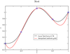
which is the smallest possible value (see Equation (18), Section 4.2, Chapter 5 of [122]). So, a grid based
on nodes of Chebyshev polynomials can be expected to perform better that a standard uniform one. This is
what can be seen in Figure 5, which shows the same function and its interpolants as in Figure 4, but with
a Chebyshev grid. Clearly, the Runge phenomenon is no longer present. One can check that,
for this choice of function  , the uniform convergence of the interpolant to the function is
recovered. This is because
, the uniform convergence of the interpolant to the function is
recovered. This is because  decreases faster than
  increases. Of
course, Faber’s result implies that this cannot be true for all the functions. There still must
exist some functions for which the interpolant does not converge uniformly to the function
itself (it is actually the class of functions that are not absolutely continuous, like the Cantor
function).
increases. Of
course, Faber’s result implies that this cannot be true for all the functions. There still must
exist some functions for which the interpolant does not converge uniformly to the function
itself (it is actually the class of functions that are not absolutely continuous, like the Cantor
function).
![N∑ | X | ΛN (X ) = maxx ∈[− 1,1] |ℓi (x)|. (23 ) i=0](article146x.gif)