In this particular section, real functions of ![]() are considered. A theorem due to Weierstrass
(see for instance [65]) states that the set
are considered. A theorem due to Weierstrass
(see for instance [65]) states that the set ![]() of all polynomials is a dense subspace of all the
continuous functions on
of all polynomials is a dense subspace of all the
continuous functions on ![]() , with the norm
, with the norm ![]() . This maximum norm is defined as
. This maximum norm is defined as
This means that, for any continuous function ![]() of
of ![]() , there exists a sequence of polynomials
, there exists a sequence of polynomials
![]() that converges uniformly towards
that converges uniformly towards ![]() :
:
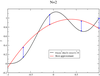
Given a continuous function ![]() , the best polynomial approximation of degree
, the best polynomial approximation of degree ![]() , is the polynomial
, is the polynomial
![]() that minimizes the norm of the difference between
that minimizes the norm of the difference between ![]() and itself:
and itself:
Chebyshev alternate theorem states that for any continuous function ![]() ,
, ![]() is unique (theorem 9.1
of [179
is unique (theorem 9.1
of [179![]() ] and theorem 23 of [150]). There exist
] and theorem 23 of [150]). There exist ![]() points
points ![]() such that the error is exactly
attained at those points in an alternate manner:
such that the error is exactly
attained at those points in an alternate manner:
| http://www.livingreviews.org/lrr-2009-1 | This work is licensed under a Creative Commons License. Problems/comments to |