Cosmological light-cone effect on the two-point correlation functions

5.1 Cosmological light-cone effect on the two-point correlation functions

Observing a distant patch of the Universe is equivalent to observing the past. Due to the finite light velocity, a line-of-sight direction of a redshift survey is along the time, as well as spatial, coordinate axis. Therefore the entire sample does not consist of objects on a constant-time hypersurface, but rather on a light-cone, i.e., a null hypersurface defined by observers at $z = 0$ . This implies that many properties of the objects change across the depth of the survey volume, including the mean density, the amplitude of spatial clustering of dark matter, the bias of luminous objects with respect to mass, and the intrinsic evolution of the absolute magnitude and spectral energy distribution. These aspects should be properly taken into account in order to extract cosmological information from observed samples of redshift surveys.

In order to predict quantitatively the two-point statistics of objects on the light-cone, one must take account of

nonlinear gravitational evolution,
linear redshift-space distortion,
nonlinear redshift-space distortion,
weighted averaging over the light-cone,
cosmological redshift-space distortion due to the geometry of the Universe, and
object-dependent clustering bias.

The Effect 5 comes from our ignorance of the correct cosmological parameters, and Effect 6 is rather sensitive to the objects which one has in mind. Thus the latter two effects will be discussed in the next Section 5.2.

Nonlinear gravitational evolution of mass density fluctuations is now well understood, at least for two-point statistics. In practice, we adopt an accurate fitting formula [67 ] for the nonlinear power spectrum $R P nl(k,z )$ in terms of its linear counterpart. If one assumes a scale-independent deterministic linear bias, furthermore, the power spectrum distorted by the peculiar velocity field is known to be well approximated by the following expression:

where $k⊥$ and $k∥$ are the comoving wavenumber perpendicular and parallel to the line-of-sight of an observer, and $(R ) Pmass(k;z)$ is the mass power spectrum in real space. The second factor on the r.h.s. comes from the linear redshift-space distortion [38 ], and the last factor is a phenomenological correction for the non-linear velocity effect [67

]. In the above, we introduce

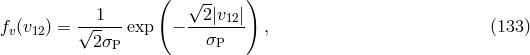
We assume that the pair-wise velocity distribution in real space is approximated by

with $σP$ being the 1-dimensional pair-wise peculiar velocity dispersion. Then the finger-of-God effect is modeled by the damping function $[ ] Dvel k∥σP (z)$ :

where $μ$ is the direction cosine in $k$ -space, and the dimensionless wavenumber $κ$ is related to the peculiar velocity dispersion $σP$ in the physical velocity units:

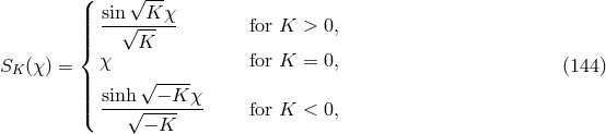
Since we are mainly interested in the scales around $1h −1 Mpc$ , we adopt the following fitting formula throughout the analysis below which better approximates the small-scale dispersions in physical units:

Integrating Equation (131 ) over $μ$ , one obtains the direction-averaged power spectrum in redshift space:

where

arctan(κ) A (κ ) = ---------, (138 ) [κ ] B (κ ) = 3-- 1 − arctan(κ)- , (139 ) κ2 κ 5 [ 3 3 arctan(κ)] C (κ ) = --2- 1 − -2-+ ------3---- . (140 ) 3κ κ κ

Adopting those approximations, the direction-averaged correlation functions on the light-cone are finally computed as

∫ zmax dVc- 2 dz dz [ϕ(z)n0 (z )] ξ(xs;z) ξLC(xs) = --zmin∫-zmax---------------------, (141 ) dzdVc-[ϕ(z)n (z)]2 zmin dz 0

where $zmin$ and $zmax$ denote the redshift range of the survey, and

Throughout the present analysis, we assume a standard Robertson–Walker metric of the form

where $SK (χ)$ is determined by the sign of the curvature $K$ as

( sin √K--χ |||| --√------ for K > 0, |{ K SK (χ) = χ for K = 0, (144 ) ||| √ ---- ||( sinh√--−-K-χ- for K < 0, − K

where the present scale factor $a0$ is normalized as unity, and the spatial curvature $K$ is given as

(see Equation (13

)). The radial comoving distance $χ(z)$ is computed by

The comoving angular diameter distance $Dc (z)$ at redshift $z$ is equivalent to $S −1(χ(z))$ , and, in the case of $Ω Λ = 0$ , is explicitly given by Mattig’s formula:

Then $dVc∕dz$ , the comoving volume element per unit solid angle, is explicitly given as