The CMB power spectrum versus experimental points

6.3 The CMB power spectrum versus experimental points

It will have become apparent in the preceding sections that the CMB data are approaching the point where meaningful comparison between theory and prediction, as regards the shape and normalisation of the power spectrum, can be made. This is particularly the case with the new availability of the recent CAT and Saskatoon results, where the combination of scales they provide is exactly right to begin tracing out the shape of the first Doppler peak. (If this exists, and if $Ωtot = 1$ .) Before embarking on this exercise, some proper cautions ought to be given. First, the current CMB data is not only noisy, with in some cases uncertain calibration, but will still have present within it residual contamination, either from the Galaxy, or from discrete radio sources, or both. Experimenters make their best efforts to remove these effects, or to choose observing strategies that minimise them, but the process of getting really ‘clean’ CMB results, free of these effects to some guaranteed level of accuracy, is still only in its infancy. Secondly, in any comparison of theory and data where parameters are to be estimated, the results for the parameters are only as good as the underlying theoretical models and assumptions that went into them. If CDM turns out not to be a viable theory for example, then the bounds on $Ω$ derived below will have to be recomputed for whatever theory replaces it. Many of the ingredients which go into the form of the power spectrum are not totally theory-specific (this includes the physics of recombination, which involves only well-understood atomic physics), so that one can hope that at least some of the results found will not change too radically.

Bearing these caveats in mind, it is certainly of interest to begin this process of quantitative comparison of CMB data with theoretical curves. Figure 21 shows

Figure 21: Analytic fit to power spectrum versus experimental points. (From Hancock et al. [35

], 1997.)

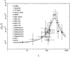
a set of recent data points, many of them discussed above, put on a common scale (which may effectively be treated as $∘ ---------- ℓ(ℓ + 1)C ℓ$ ), and compared with an analytical representation of the first Doppler peak in a CDM model. The work required to convert the data to this common framework is substantial, and is discussed in Hancock et al. (1997) [35 ], from where this figure was taken. The analytical version of the power spectrum is parameterised by its location in height and left/right position, and enables one to construct a likelihood surface for the parameters $Ω$ and $Apeak$ , where $Apeak$ is the height of the peak, and is related to a combination of $Ωb$ and $H0$ , as discussed above. The dotted and dashed extreme curves in Figure 21 indicate the best fit curves corresponding to varying the Saskatoon calibration by ±14%. The central fit yields a 68% confidence interval of

with a maximum likelihood point of $Ω = 0.7$ after marginalisation over the value of $Apeak$ . Incorporating nucleosynthesis information as well, as sketched above (specifically the Copi et al. [22 ] bounds of $0.009 ≤ Ωbh2 ≤ 0.02$ are assumed), a 68% confidence interval for $H0$ of

is obtained. This range ignores the Saskatoon calibration uncertainty. Generally, in the range of parameters of current interest, increasing $H0$ lowers the height of the peak. Thus taking the Saskatoon calibration to be lower than nominal, for example by the 14% figure quoted as the one-sigma error, enables us to raise the allowed range for $H0$ . By this means, an upper limit closer to 70 km s^–1 Mpc^–1 is obtained.

The best angular resolution offered by MAP is 12 arcmin, in its highest frequency channel at 90 GHz, and the median resolution of its channels is more like 30 arcmin. This means that it may have difficulty in pining down the full shape of the first and certainly secondary Doppler peaks in the power spectrum. On the other hand, the angular resolution of the Planck Surveyor extends down to 5 arcmin, with a median (across the six channels most useful for CMB work) of about 10 arcmin. This means that it will be able to determine the power spectrum to good accuracy, all the way into the secondary peaks, and that consequently very good accuracy in determining cosmological parameters will be possible. Figure 19 , taken from the Planck Surveyor Phase A study document, shows the accuracy to which $Ω$ , $H0$ and $Ωb$ can be recovered, given coverage of 1/3 of the sky with sensitivity 2 × 10^–6 in $ΔT ∕T$ per pixel. The horizontal scale represents the resolution of the satellite. From this we can see that the good angular resolution of the Planck Surveyor should mean a joint determination of $Ω$ and $H0$ to $∼$ 1% accuracy is possible in principle. Figure 22 show the likelihood contours for two experiments with different resolutions.

Figure 22: The contours show 50, 5, 2 and 0.1 percentile likelihood contours for pairs of parameters determined from fits to the CMB power spectrum. The figures to the left show results for an experiment with resolution $∘ 𝜃FWHM = 1$ . Those to the right for a higher resolution experiment with $′ 𝜃FWHM = 10$ plotted on the same scale (central column) and with expanded scales (rightmost column). This figure is taken from Bersanelli et al. 1996 [10 ].

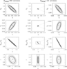
These figures do not, however, take into account any reduction in sensitivity as a result of the need to separate Galactic foregrounds from the CMB. Nevertheless, simulations using a maximum entropy separation algorithm (Hobson, Jones, Lasenby & Bouchet, in press) suggest that for the Planck Surveyor the reduction in the final sensitivity to the CMB is very small indeed, and that the accuracy of the cosmological parameters estimates indicated in Figure 19 may be attainable.

One additional problem is that of degeneracy. It is possible to formulate two models with similar power spectra, but different underlying physics. For example, standard CDM and a model with a non zero cosmological component and a gravity wave component can have almost identical power spectra (to within the accuracy of the MAP satellite). To break the degeneracy more accuracy is required (like the Planck Surveyor) or information about the polarisation of the CMB photons can be used. This extra information on polarisation is very good at discriminating between theories but requires very sensitive polarimeters.