Linear growth rate of the density fluctuation

2.7 Linear growth rate of the density fluctuation

Most likely our Universe is dominated by collisionless dark matter, and thus $λJ$ is negligibly small. Thus, at most scales of cosmological interest, Equation (54

) is well approximated as

For a given set of cosmological parameters, one can solve the above equation by substituting the expansion law for $a(t)$ as described in Section 2.3. Since Equation (55

) is the second-order differential equation with respect to $t$ , there are two independent solutions; a decaying mode and a growing mode which monotonically decreases and increases as $t$ , respectively. The former mode becomes negligibly small as the Universe expands, and thus one is usually interested in the growing mode alone.

More specifically those solutions are explicitly obtained as follows. First note that the l.h.s. of Equation (18 ) is the Hubble parameter at $t$ , $H (t) = a˙∕a$ :

( Ωm 1 − Ωm − Ω Λ ) H2 = H20 --3-+ -------2----- + Ω Λ (56 ) [ a a ] = H20 Ωm (1 + z)3 + (1 − Ωm − Ω Λ)(1 + z)2 + Ω Λ . (57 )

The first and second differentiation of Equation (56

) with respect to $t$ yields

and

respectively. Thus the differential equation for $H$ reduces to

This coincides with the linear perturbation equation for $δk$ , Equation (55

). Since $H (t)$ is a decreasing function of $t$ , this implies that $H (t)$ is the decaying solution for Equation (55

). Then the corresponding growing solution $D (t)$ can be obtained according to the standard procedure: Subtracting Equation (55

) from Equation (60

) yields

and therefore the formal expression for the growing solution in linear theory is

It is often more useful to rewrite $D (t)$ in terms of the redshift $z$ as follows:

where the proportional factor is chosen so as to reproduce $D (z) → 1∕(1 + z)$ for $z → ∞$ . Linear growth rates for the models described in Section 2.3 are summarized below:

Einstein–de Sitter model ( $Ω = 1,Ω = 0 m Λ$ ):
Open model with vanishing cosmological constant ( $Ωm < 1, ΩΛ = 0$ ):
Spatially-flat model with cosmological constant ( $Ωm < 1,Ω Λ = 1 − Ωm$ ):

For most purposes, the following fitting formulae [67 ] provide sufficiently accurate approximations:

g(z) D (z) = ------, (67 ) 1 + z 5Ω-(z)---------------------1-------------------- g(z) = 2 Ω4 ∕7(z ) − λ (z ) + [1 + Ω(z)∕2][1 + λ(z)∕70], (68 )

where

[ ]2 3 Ω (z) = Ωm (1 + z)3 -H0-- = ---------------Ωm-(1 +-z)----------------, (69 ) H (z) Ωm (1 + z)3 + (1 − Ωm − ΩΛ )(1 + z)2 + Ω Λ [ H ]2 Ω λ(z) = ΩΛ ---0- = ----------3----------Λ------------2------. (70 ) H (z) Ωm (1 + z) + (1 − Ωm − Ω Λ)(1 + z ) + Ω Λ

Note that $Ωm$ and $ΩΛ$ refer to the present values of the density parameter and the dimensionless cosmological constant, respectively, which will be frequently used in the rest of the review.

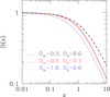
Figure 2 shows the comparison of the numerically computed growth rate (thick lines) against the above fitting formulae (thin lines), which are practically indistinguishable.

Figure 2: Linear growth rate of density fluctuations.